Matthew Berry, New York Times bestselling author and mediocre fantasy football advice-giver (this is a compliment; you have to listen to the podcast), does a column each year called “100 Facts.”  In his intro, each time, he warns about the exercise he is going to undertake.  Statistics can be shaded in whatever way you wish (I’m paraphrasing him), so he acknowledges that he is presenting the best facts to support his perceptions of players.  But he goes further to say that’s all other fantasy football analysts are doing as well – he’s just the one being honest about it.  It’s the analyst’s equivalent of Penn and Teller’s cups and ball trick with clear cups – just because you know how the trick is done doesn’t make it less entertaining.

With the knowledge of statistics comes the responsibility of presenting them effectively.  My first and much beloved nonprofit boss used to say that if you interrogate the data, it will confess.  I would humbly submit a corollary: if you torture the data, it will start confessing to stuff just to make you stop.

A well-wrapped statistic is better than Hitler’s “big lie”; it misleads, yet it cannot be pinned on you.
— How to Lie with Statistics by Darrell Huff

So here are some common tricks people will use to make their points.  Arm yourself against this, less you be the victim of data presented with either malice or ignorance.

The wonky y-axis

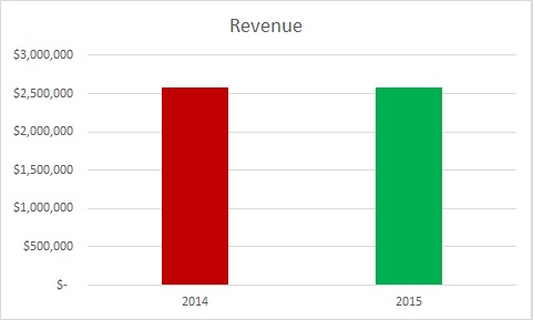
The person presenting to you was supposed to increase revenue by a lot.  In fact, s/he increased it by only a little.  The weasel solution?  Make a mountain out of that molehill:

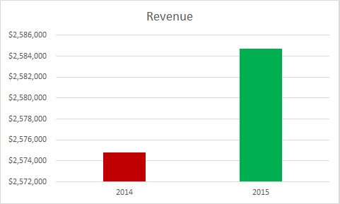
Note that the difference between the top and bottom of the y-axis is only $10,000.  Here’s what that same graph looks like with the y-axis starting at 0, as we are trained to expect unless there’s a very good reason:

Both are true, but the latter is a more accurate representation of what went on over the year.

Ignoring reference points

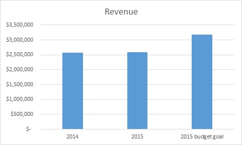
Let’s take a look at that last graph with the budgeted goal added in.

This tells a very different story, no? Always be on the lookout for context like this.

The double wonky y-axis

I’ve been saving a Congressional slide for this blog post.  I make no claims about which side of this issue is true or right or moral or whatever.  That said, this is also a good example of having quality debates with good data versus intentionally putting your spin on the ball.

This graph was presented by Congressman Jason Chaffetz in the debate over Planned Parenthood.

Hat tip to PolitiFact.

The graph seems to say that Planned Parenthood health screenings have decreased, abortions have increased, and now Planned Parenthood performs more abortions than health screenings.

But this is a case where the graph has two different y-axes.  Looking at the data, you can see that there were still well more than double as many prevention services performed as abortions.  When we look at the graph, it looks like the opposite is true.

Again, you may choose to do with this information what you will; there are many who would say one abortion is too many.  However, to paraphrase Daniel Patrick Moynihan, you can have your own opinions, but not your own facts.

The outliers

This is one of those things that is less frequently used by people to fool you and more often overlooked by people who subsequently fool themselves.

Here’s a sample testing report.

This one seems like a pretty clean win for Team Test Letter.  Generally, you are going to take the .2% point decrease in response rate in order to increase average gift by $7 and an additional 14.6 cents per piece mailed out.  Game, set, match.

But one must always ask the uber-question, why. So you look at the donations. It turns out a board member mailed her annual $10,000 gift to the test package.  No such oddball gifts went to the control package.  Since this is not likely a replicable event, let’s take out this one chance donation out and look at the data again.
An even cleaner win for Team Control.  The test appears to have suppressed both response rate and average gift.

Percentages versus absolutes

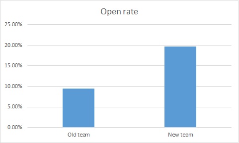
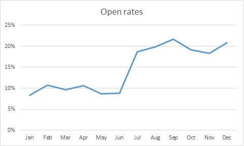
Check out the attached graph of email open rates, where a new online team came it and the director bragged about the increase in open rates.  I actually saw a variant of this one happen live.

Wow.  Clearly, much better subject lines under the new regime, no?  More people are getting our messages.

Well, for clarity, let’s look at this on a month by month basis.

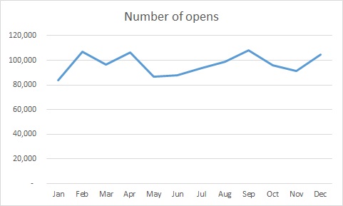
So, something happened in July that spiked open rates. Maybe it’s the new team, but we must ask why. One of the common culprits, when you are looking at percentages, is a change in N, the denominator.  Let’s look at the same graph, but instead of percentages, we are going to look at the number of people who opened the email.

Huh.  Our big spike disappeared.

In looking into this, July is when we started suppressing people who had not opened an email in the past six months.  This is actually a very strong practice, preventing people who don’t want to get email from you, have moved on to another address, or were junk data to begin with off of your files.  As a result, your likelihood of being called spam goes down significantly.

So it wasn’t that twice as many people were opening emails; it was that half as many people (the good half) were getting the emails.

Correlation does not equal causation

The wonderful site FiveThirtyEight recently did a piece on how Matt Damon is more attractive in movies where he is perceived as being smarter.  For example, see how dreamy Damon is perceived to be as super-genius Will Hunting.  As Irene Adler says to Sherlock in the eponymous BBC series, brainy is the new sexy.

And you can look at this and think a logical conclusion: the smarter a Matt Damon character is in a movie, the more attractive that character is perceived to be.  This is plausible even though dreaminess was judged from a still frame – if Matt Damon is wearing an attractive sweater, it’s one of the Bourne movies; if it’s WWII garb, probably Saving Private Ryan.

This conclusion would reason that when Damon plays Neil DeGrasse Tyson in the upcoming biopic, his resultant sexiness will distract from the physical mismatching casting.

There’s also the hypothesis posited by the author: “The more attractive Damon is perceived to be in a movie, the smarter he is perceived to be.”  This says the reverse of the above: if Damon is attractive in a movie, he will be perceived to be smart.  This too is plausible – we tend to overestimate the competence of people we find to be attractive (hence why there is no picture of me on the site – you would immediately start discounting my advice).

Or it could be an exogenous third factor that causes both.  What if make-up artists want to symbolize dumbness by making actors unattractive (actually, since it’s Matt Damon, let’s say less attractive not unattractive)?  Film is after all a visual medium and since they know people underestimate less attractive people, they aim to make less competent characters less attractive.

Those are the ways correlation can go: A can cause B, B can cause A, or C can cause A and B.

This is what we must guard against in drawing final conclusions, but rather continually refined theories.  Let’s say you are seeing a general trend that your advocacy mail packages are doing better than your average mail package.  It’s generally safe to say more advocacy mail packages would be better.  But what if it isn’t the advocacy messaging, but that advocacy messages have a compelling reply device?  Or that when you mailed your advocacy pieces, you were also in the news?

One of the key parts of determining the results of a test is learning what the test actually means.  It’s important to strip away other possibilities until you have determined what the real mechanism is for success or failure.  This is why, for the blog analysis last week, I did a regression analysis rather than a series of correlations – to control for autocorrelations.

You don’t have to be versed in all manner of stats; the most important thing it to keep asking why.  From that, you can find the closest version to the truth.